Table Of Content
The first independent variable is light switch #1, and it has two levels, up or down. The second independent variable is light switch #2, and it also has two levels, up or down. When there are two independent variables, each with two levels, there are four total conditions that can be tested. Another common approach to including multiple dependent variables is to operationalize and measure the same construct, or closely related ones, in different ways. Imagine, for example, that a researcher conducts an experiment on the effect of daily exercise on stress.
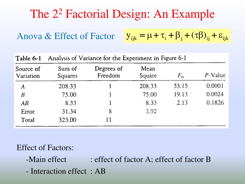
A Note about Factors with 4 levels - \(2^2\)
One independent variable was disgust, which the researchers manipulated by testing participants in a clean room or a messy room. The other was private body consciousness, a participant variable which the researchers simply measured. Another example is a study by Halle Brown and colleagues in which participants were exposed to several words that they were later asked to recall (Brown, Kosslyn, Delamater, Fama, & Barsky, 1999)[1]. Some were negative health-related words (e.g., tumor, coronary), and others were not health related (e.g., election, geometry). The nonmanipulated independent variable was whether participants were high or low in hypochondriasis (excessive concern with ordinary bodily symptoms). The result of this study was that the participants high in hypochondriasis were better than those low in hypochondriasis at recalling the health-related words, but they were no better at recalling the non-health-related words.
Book traversal links for 13.3 - The Two Factor Mixed Models
Instead, the experimenter changes the levels of the independent variable and then observes possible changes in the measures. This kind of design has a special property that makes it a factorial design. That is, the levels of each independent variable are each manipulated across the levels of the other indpendent variable. In other words, we manipulate whether switch #1 is up or down when switch #2 is up, and when switch numebr #2 is down.
2. Mixed Factorial ANOVA as a mixed-effect model…
G., to collect interview data and survey data of one inquiry simultaneously; in that case, the research activities would be concurrent. It is also possible to conduct the interviews after the survey data have been collected (or vice versa); in that case, research activities are performed sequentially. Similarly, a study with the purpose of expansion can be designed in which data on an effect and the intervention process are collected simultaneously, or they can be collected sequentially. We leave it to the reader to decide if he or she desires to conduct a qualitatively driven study, a quantitatively driven study, or an equal-status/“interactive” study. According to the philosophies of pragmatism (Johnson and Onwuegbuzie 2004) and dialectical pluralism (Johnson 2017), interactive mixed methods research is very much a possibility. By successfully conducting an equal-status study, the pragmatist researcher shows that paradigms can be mixed or combined, and that the incompatibility thesis does not always apply to research practice.
α-Fe2O3/Nb2O5 mixed oxide active for the photodegradation of organic contaminant in water: Factorial experimental ... - ScienceDirect.com
α-Fe2O3/Nb2O5 mixed oxide active for the photodegradation of organic contaminant in water: Factorial experimental ....
Posted: Sat, 02 Nov 2019 06:56:32 GMT [source]
Time of day (day vs. night) is represented by different locations on the x-axis, and cell phone use (no vs. yes) is represented by different-colored bars. It would also be possible to represent cell phone use on the x-axis and time of day as different-colored bars. The choice comes down to which way seems to communicate the results most clearly. The bottom panel of Figure 5.3 shows the results of a 4 x 2 design in which one of the variables is quantitative.
How to Construct a Mixed Methods Research Design
(e) Confirm and discover – this entails using qualitative data to generate hypotheses and using quantitative research to test them within a single project. The ezANOVA() function provides us with more detail, for instanceautomatically providing Mauchly’s Test for Sphericity and both theGreenhouse-Geisser and Hyunh-Feldt corrections in the event that thesphericity assumption is violated. Most importantly, however, theoutputs of these two functions agree when we look at the f-statisticsfor all main-effects and interactions when sphericity is assumed.
But by ruling out some of the most plausible third variables, the researchers made a stronger case for SES as the cause of the greater generosity. The difference between red and green bars is small for level 1 of IV1, but large for level 2. The differences between the differences are different, so there is an interaction. For example, both the red and green bars for IV1 level 1 are higher than IV1 Level 2.
Simplest reaction time analysis for experimental psychology? - ResearchGate
Simplest reaction time analysis for experimental psychology?.
Posted: Fri, 29 Mar 2019 07:00:00 GMT [source]
This variable, psychotherapy length, is represented along the x-axis, and the other variable (psychotherapy type) is represented by differently formatted lines. This is a line graph rather than a bar graph because the variable on the x-axis is quantitative with a small number of distinct levels. The research designs we have considered so far have been simple—focusing on a question about one variable or about a statistical relationship between two variables.

2 - \(3^k\) Designs in \(3^p\) Blocks cont'd.
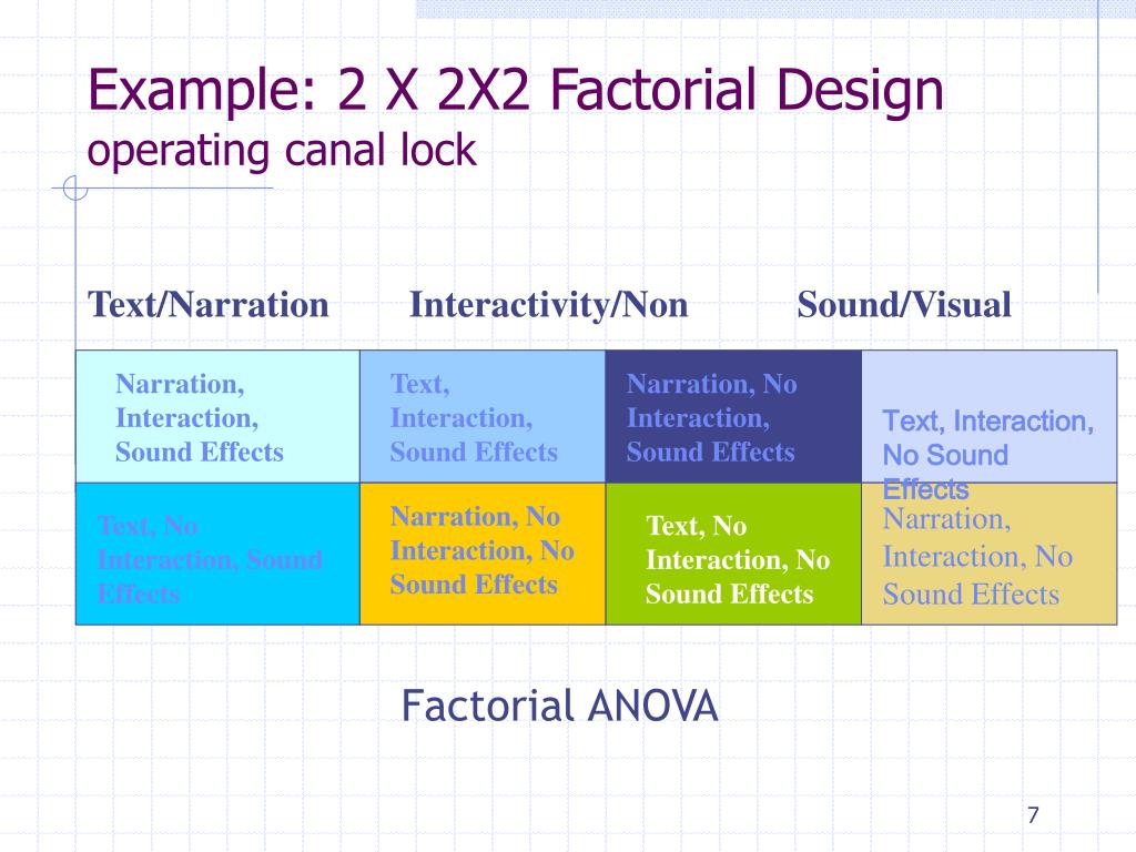
If they were low in private body consciousness, then whether the room was clean or messy did not matter. There is an interaction effect (or just “interaction”) when the effect of one independent variable depends on the level of another. A 2×2 factorial design is a type of experimental design that allows researchers to understand the effects of two independent variables (each with two levels) on a single dependent variable. An approach to including multiple independent variables in an experiment where each level of one independent variable is combined with each level of the others to produce all possible combinations. Often a researcher wants to know how an independent variable affects several distinct dependent variables. As another example, researcher Susan Knasko was interested in how different odors affect people’s behavior [Kna92].
But it could also be that the music was ineffective at putting participants in happy or sad moods. A manipulation check, in this case, a measure of participants’ moods, would help resolve this uncertainty. If it showed that you had successfully manipulated participants’ moods, then it would appear that there is indeed no effect of mood on memory for childhood events. But if it showed that you did not successfully manipulate participants’ moods, then it would appear that you need a more effective manipulation to answer your research question. Again, because neither independent variable in this example was manipulated, it is a cross-sectional study rather than an experiment.
It’s when you become highly irritated and angry because you are very hungry…hangry. I will propose an experiment to measure conditions that are required to produce hangriness. The pretend experiment will measure hangriness (we ask people how hangry they are on a scale from 1-10, with 10 being most hangry, and 0 being not hangry at all). The first independent variable will be time since last meal (1 hour vs. 5 hours), and the second independent variable will be how tired someone is (not tired vs very tired). When the independent variable is a construct that can only be manipulated indirectly—such as emotions and other internal states—an additional measure of that independent variable is often included as a manipulation check.
In other words, the effect of wearing a shoe does not depend on wearing a hat. More formally, this means that the shoe and hat independent variables do not interact. It would mean that the effect of wearing a shoe on height would depend on wearing a hat. But in some other imaginary universe, it could mean, for example, that wearing a shoe adds 1 to your height when you do not wear a hat, but adds more than 1 inch (or less than 1 inch) when you do wear a hat. This thought experiment will be our entry point into discussing interactions. A take-home message before we begin is that some independent variables (like shoes and hats) do not interact; however, there are many other independent variables that do.
If you do this, then you simply have a single-factor design, and you are asking whether that single factor caused change in the measurement. For a 2x2 experiment, you do this twice, once for each independent variable. The number of possible purposes for mixing is very large and is increasing; hence, it is not possible to provide an exhaustive list. Greene et al.’s (1989) purposes, Bryman’s (2006) rationales, and our examples of a diversity of views were formulated as classifications on the basis of examination of many existing research studies. They indicate how the qualitative and quantitative research components of a study relate to each other. These purposes can be used post hoc to classify research or a priori in the design of a new study.
The dependent variable, stress, is a construct that can be operationalized in different ways. For this reason, the researcher might have participants complete the paper-and-pencil Perceived Stress Scale and also measure their levels of the stress hormone cortisol. If the researcher finds that the different measures are affected by exercise in the same way, then he or she can be confident in the conclusion that exercise affects the more general construct of stress. Even if you are primarily interested in the relationship between an independent variable and one primary dependent variable, there are usually several more questions that you can answer easily by including multiple dependent variables. Most complex correlational research, however, does not fit neatly into a factorial design. Instead, it involves measuring several variables, often both categorical and quantitative, and then assessing the statistical relationships among them.
These included health, knowledge of heart attack risk factors, and beliefs about their own risk of having a heart attack. They found that more optimistic participants were healthier (e.g., they exercised more and had lower blood pressure), knew about heart attack risk factors, and correctly believed their own risk to be lower than that of their peers. When multiple dependent variables are different measures of the same construct - especially if they are measured on the same scale - researchers have the option of combining them into a single measure of that construct. Recall that Schnall and her colleagues were interested in the harshness of people’s moral judgments. To measure this construct, they presented their participants with seven different scenarios describing morally questionable behaviors and asked them to rate the moral acceptability of each one. Although the researchers could have treated each of the seven ratings as a separate dependent variable, these researchers combined them into a single dependent variable by computing their mean.


No comments:
Post a Comment